Weather forecasts are calculated by computer models (or dynamical models) that describe the evolution of the real atmosphere using mathematical equations. But, did you know that there are two distinct types of forecasts created from these models? In this article we explore four topics and explain the difference between deterministic and ensemble forecasts:
- How models work,
- The deterministic forecast,
- The ensemble forecast,
- The relative merits of each method.
The Difference Between Deterministic and Ensemble Forecasts: How Models Work
The equations at the heart of a dynamical model are designed to digitally mimic the natural processes at work in the atmosphere all around the globe. For example, Newton’s second law forms an important backbone to the equations of atmospheric motion. It’s usually written as
F=ma,
and stated as “Force equals mass times acceleration”.
To apply Newton’s second law to weather forecasting, however, we use the form:
a=F/m.
In plain language, the acceleration of air is equal to the forces acting on it divided by air’s mass. This form of Newton’s second law makes weather modelling possible! The forces include pressure gradients, gravity, and Coriolis forces owing to the Earth’s rotation, and friction.
Utilizing this type of equation is achieved by using a grid containing millions of data points positioned at regular intervals in a virtual, computer-based world. The most complex models replicate atmospheric processes such as rainfall, the underlying land and ocean surfaces, as well as the various forms of incoming and outgoing energy (i.e. sunlight, amongst others).
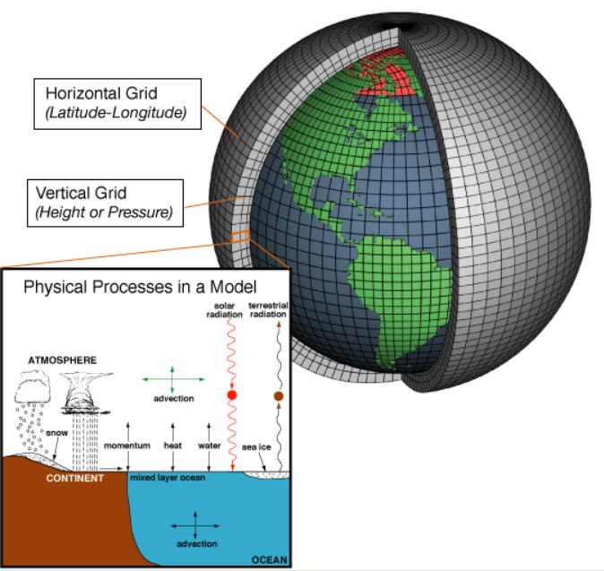
Before we can set our model to work, the computer needs to know the current state of the atmosphere, which is referred to as the initial conditions (IC). Observational data from sources such as satellites, surface weather stations, weather balloons, and aircraft readings are usually refreshed and input into the model every 12 hours.
Once the IC are set, the computer gets to work on calculating the forecast; solving the basic equations of motion and energy across the whole globe. The model steps forward in time many days into the future, producing forecast values for variables such as temperature, wind, and rainfall.

Deterministic Forecast
In order to understand the difference between deterministic and ensemble forecasts, we need to know more about deterministic forecasts. When a dynamical model runs once at the highest possible resolution – which means it uses all of the available computing power to create the forecast, the forecast produced is known as a deterministic forecast (DF).
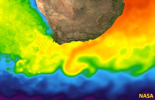
This type of forecast represents atmospheric processes in the finest possible detail, and thus generates a relatively detailed forecast (Figure 2). But, because of the uncertainty of the initial conditions, the deterministic forecast is only one possible future outcome of an infinite number of possibilities.
The DF typically performs very well in the first six days ahead, but it can become unreliable at the seven to ten-day lead times, often showing an increasingly unlikely evolution.
There are two main sources of forecast error. The first source arises because the equations in the model do not perfectly replicate all of the natural processes at work in the atmosphere.
The second occurs because the computer model knows surprisingly little about the real world. The observational data used to construct the IC represents just a fraction of the information contained in the real atmosphere.
These initial errors become increasingly large as the forecast moves forward in time. This problem is often referred to as the butterfly effect. Technically, the butterfly effect is a sensitive dependence to initial conditions that can cause the model solution to be substantially different from the real world when the forecast calculation starts – the phrase implies that the flap of a butterfly’s wings could significantly change the forecast. That means small discrepancies between the weather forecast model initial conditions and the real-world conditions cause the forecast error to grow uncontrollably. The error will eventually grow so large that a deterministic forecast is no longer useful.
Another drawback of a deterministic forecast is that it provides only a single forecast; it gives no suggestion of alternatives, or any indication of forecast uncertainty. It provides the user with no indication of the confidence to place on the forecast.
Ensemble Forecast
In order to understand the difference between deterministic and ensemble forecasts, we need to know more about ensemble forecasts. At many weather modeling centers, as soon as the computer has finished processing the DF, it gets to work on the second type of forecast; an Ensemble Forecast. As the name suggests, the ensemble is comprised of many forecasts or members – anywhere between 12 and 51, depending on the center.
In Figure 3 time moves left to right; the DF is shown by the single bold line, and the many forecasts of the ensemble are shown by the dashed lines. As the power of the computer is fixed, and the 12 to 51 ensemble members are calculated concurrently, the forecasts are necessarily run at a much lower resolution than the deterministic forecast.
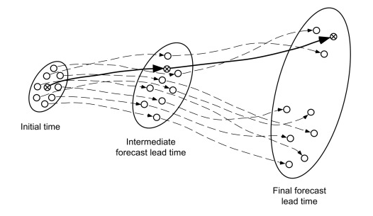
But why do we do this? As you might expect, if we run the same model twice, with precisely the same IC, then it produces two identical forecasts, which is of no use whatsoever.
To produce a set of ensemble forecasts, the IC are changed slightly for each ensemble member. There is uncertainty in the original IC and the new IC are just as likely to match the real world as those used for the DF – this is known as sampling the uncertainty (the different starting points are shown on the left of the image in Figure 3). In some models, slight variations are also made to the equations in an attempt to capture some of the model uncertainty.
The advantage gained in producing many possible outcomes outweighs the fact that the ensemble members are run at lower resolution – and the Ensemble Average (EA) is often more skillful than the DF at longer lead times. In fact, an ensemble forecast is a vital tool for long range forecasting.
The ensemble forecast is a little more challenging to work with than a deterministic forecast;
- Interpreting multiple forecasts can be complex, so very often the EA is used for simplicity.
- As the ensemble runs at a lower resolution than the DF, it is less sensitive to changes in the IC and thus can be slower to respond to new observations.
The critical advantage of the ensemble forecast is that it provides probabilities of what may occur as the atmosphere evolves. If the ensemble members are quite similar at a point and time, the forecast is more likely to be skillful than if the members are widely separated. And thus the ensemble approach not only provides a forecast, it also provides an indication of the skill of the forecast.
Ensemble Forecast Output
Figure 4 shows a typical box and whisker plot of daily temperature in the ensemble forecast, where time advances left to right. The various heights of the boxes indicate 100% of the range, 80% of the range, 50% of the range, and the median is the central bar (which is similar to the EA).
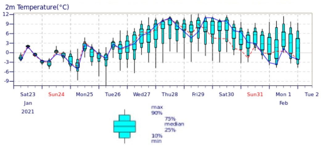
In weather forecasting, confidence means how likely the forecast is to be correct. We can see that early in the forecast (left side of graph Figure 4), the small boxes indicate a narrow range of possibilities and thus confidence is high. As we move forward in time (towards the right side of graph Figure 4) then the boxes become much taller, indicating much lower confidence in the forecast.
If the model is calibrated in such a way that the range of temperatures generated by the ensemble model matches the range of temperatures seen in the real world, and any bias is removed, then we find the model produces reliable forecasts.
Reliable forecasts are very powerful; if the forecast says there is a 50-60 percent chance of an event, then it is sure to happen 50-60 percent of the time.
Forecasts framed in terms of probabilities may be difficult for people to process, but they do lend themselves well to numerical contingency models, which are used for example, in agricultural planning, and in energy pricing models.
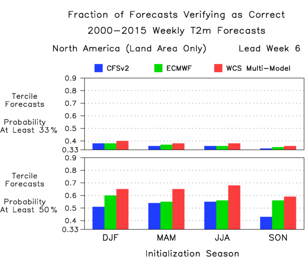
As mentioned earlier, probabilistic output lends itself very well to long range forecasting. Some models have been shown to possess skill as far as six weeks into the future (Figure 5).
Why Ensemble Forecasting Improves Forecast Skill
Recall two important points from the discussion above. The first is that a weather forecast is based on the initial conditions of the forecast, which contains a version of the information necessary for the mathematical equations to run forward in time. Weather forecasting is an initial condition problem.
The second is that the butterfly effect means that small errors in those initial conditions grow with increasing lead time and eventually become so large the forecast has no skill. When this occurs the noise (i.e., the error) is much larger than the signal.
Ensemble forecasting provides an opportunity to minimize the forecast error while extracting the signal from the forecast. By averaging over many possible future forecast realizations (i.e., each ensemble member) the errors tend to cancel one another out.
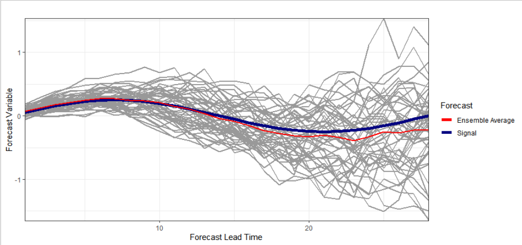
The benefits of ensemble forecasting are shown in Figure 6. The error of any individual ensemble member increases over time. However, by averaging all ensemble members together a close approximation to the actual signal emerges.
In this simple example, we are averaging the forecast ensemble for each day of the forecast. Long-range forecasts achieve additional signal identification by also averaging over time. For example, averaging the ensemble forecast from the day 15 to 21 and day 22 to 28 would provide a three- and four-week lead forecast, respectively.
Figure 6 also shows that the forecast uncertainty increases with forecast lead time. This information is also used to estimate the probability of a specific outcome. When applied within the context of the World Climate Service, it provides tercile forecasts of below normal, normal, and above normal conditions. The forecasts are calibrated such that the probability forecasted reflects the frequency with which the event will occur in reality.
Skill of Deterministic Forecasts vs Ensemble Forecasts
Here is a difference between deterministic and ensemble forecasts. The highly detailed deterministic forecast is able to resolve small scale features, and this precision scores very well in the early stages of the forecast as the model closely matches the real world. As time progresses, the small-scale features in the model start to misalign with the equivalent features in the real world. As the model continues to give very specific weather values and locations, this precision becomes detrimental, and accuracy drops rapidly at around 6 days ahead as the noise starts to become larger than the signal (Figure 7).
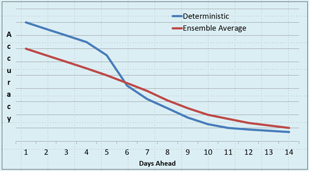
In the lower resolution ensemble forecast, the model is relatively vague about values and positions and thus accuracy is modest. As time progresses, accuracy declines at a steady rate. Beyond six days ahead, the vagueness of the EA works to its advantage and makes the forecast a better guide than the deterministic forecast.
We see that the best forecast is given by the DF in the early stages of the evolution, but where the lines cross at around 6 days ahead, so the ensemble becomes the more accurate model. In this way, the model that gives the better forecast is determined by the horizon for which we are forecasting.
The Difference Between Deterministic and Ensemble Forecasts: Conclusion
In this article we have explored the difference between deterministic and ensemble forecasts.
The deterministic forecast consists of one forecast which has high resolution, is easy to use, shows good accuracy in the first six days, and is sensitive to new data. It gives no indication of confidence, it cannot produce probability forecasts, and has little skill in the long range.
The ensemble forecast consists of many forecasts which have lower resolution: it can be complicated to use, it is usually best for longer lead times, and does not always respond rapidly to new data. It does provide forecast confidence, predicts weather variables in terms of probabilities, and can be more skilful in the long range.