Ensemble forecasts form an essential part of long-range weather forecasting. In this article we take a peek under the hood of the invaluable ensemble.
Ensemble Forecast: Introduction
Short-range weather forecasting has traditionally relied on a single, high-resolution model simulation known as a deterministic forecast. Small initial errors in the observed initial conditions in deterministic models quickly amplify such that the signal is lost within the noise beyond approximately seven days into the future. Ensembles (multiple forecasts) were developed in the late 1980s to overcome this constraint. This article looks at what an ensemble forecast is and how they are useful in the medium to long-range forecast timeframe.
Ensemble Forecast: How an Ensemble Forecast is Produced
As the name suggests, an ensemble forecast is comprised of many forecasts or members. Modern ensemble forecasts have anywhere between 12 and 51 members, depending on the model. As the power of the computer is limited and the ensemble members are calculated concurrently, the forecasts are necessarily run at a much lower spatial resolution than a deterministic model.
To ensure that each member of the ensemble is unique, the initial weather values, or initial conditions (IC), are changed slightly and differently to start the forecast of each ensemble member. As there is uncertainty in the original IC, the new IC is just as likely to predict the actual weather as other members. In other words, each ensemble member forecasts weather conditions that are equally likely in the future. Thus, this technique estimates the uncertainty of a forecast. In some models, slight variations are made to the model equations attempting to capture some of the model physics uncertainty.
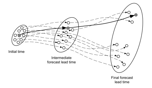
In Figure 1 we see members starting from different initial conditions depicted in the circle on the left. As time elapses (left to right), each forecast follows its own unique path to some new set of values in the future. Each forecast is equally as likely to be correct as any other forecast. We see that the ensemble produces a range of possible outcomes rather than producing a single outcome.

Ensemble Forecast: Model Output
The advantage gained in producing an ensemble of many possible outcomes outweighs the fact that each ensemble member is run at a lower resolution than a deterministic forecast; the average of all of the ensemble members is more skilful than any single forecast at lead times beyond seven days.
The ensemble forecasts can be challenging to interpret because each forecast is a group of numbers rather than a single value. The average of the ensemble at each place and time—a single forecast value—is often used for simplicity, but this method overlooks a unique property of ensemble forecasts.
The range or spread of forecasts produced by the ensemble provides additional and valuable data about the uncertainty of the forecast. The forecast spread enables the user to see the breadth of possible outcomes and thus the likelihood of various weather events. This unique property of ensemble forecasts provides a useful way to measure uncertainty in the forecast.
Ensemble Forecast: Confidence
Figure 2 shows a typical box and whisker plot of daily temperature in the ensemble forecast, in which time advances from left to right. The various heights of the boxes indicate 100 percent, 80 percent, and 50 percent of the forecast range. The median of the forecast is denoted by the central bar (which is similar to the ensemble average).
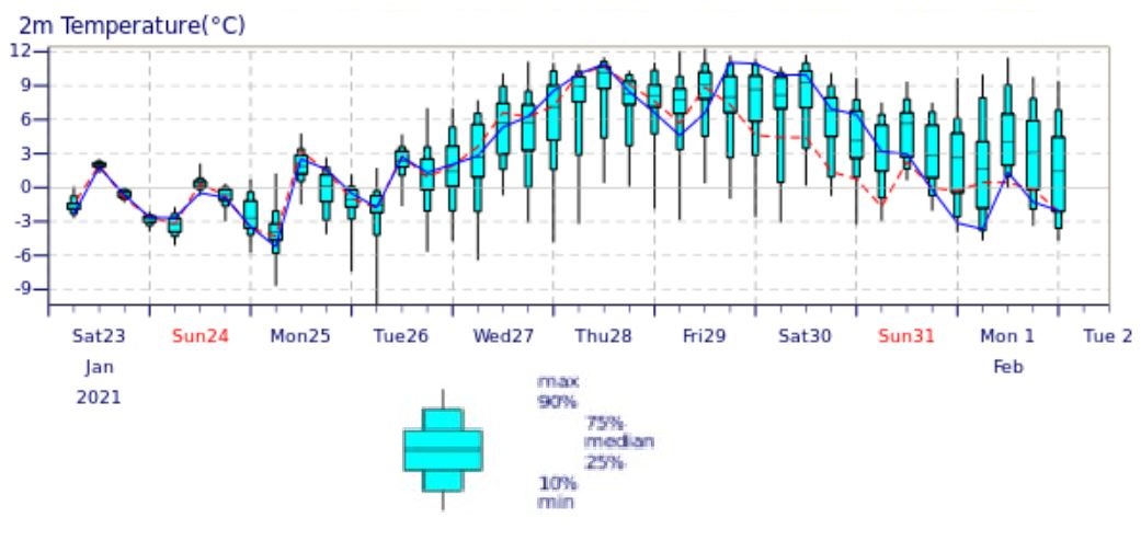
The confidence of a weather forecast denotes how likely the forecast is to be correct. Early in the above forecast (left-side of Figure 2), the small boxes indicate a narrow range of possibilities. Therefore, the forecast confidence is high. Moving forward in time (towards the right side of Figure 2), the boxes become much taller, indicating greater forecast uncertainty and a lower confidence forecast.
Ensemble forecasts are improved through a process called calibration [link]. Calibration compares a history of ensemble forecasts to the historical weather conditions that were previously forecast. The comparison allows the model uncertainty to be improved and corrected such that the range of temperatures over many forecasts matches the range of temperatures seen in the real world. In addition, forecast bias, which is average differences between the model forecast and observed conditions, is removed. Thus, calibration ensures the model produces reliable forecasts.
Reliable forecasts are very powerful; if the forecast says there is a 40 percent chance of an event, then it will happen at least 40 percent of the time.
Forecasts framed in terms of probabilities may be difficult for people to understand, but they do lend themselves well to numerical contingency models, which are valuable in a wide range of planning applications, including agriculture and energy pricing models.
Ensemble Forecast: Long-Range Forecasting
As we have discussed, ensemble forecasting is an essential tool for medium to long-range forecasting. Ensemble forecasting enables skillful forecasts to be made well beyond the 10 to 14-day medium-range forecast. Capturing long-range forecast skill requires the forecast information to be averaged over several days rather than individual days. For example, the World Climate Service produces long-range forecasts for target weeks, be that a calendar week, business week, or US Energy Information Administration week.
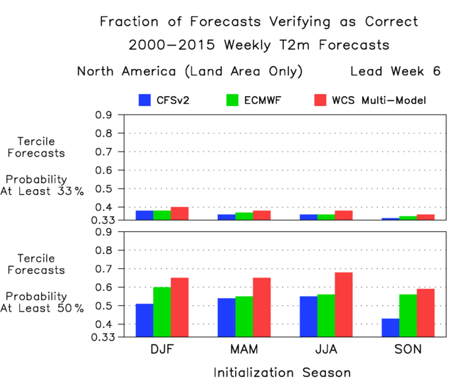
The WCS calibrates ensemble forecasts to produce reliable long-range forecasts. The output is split into three equally likely categories or terciles; above normal, near normal, and below normal. The image below shows that some temperature forecasts of above or below normal temperatures for six weeks ahead can have a 50-60 percent likelihood of being correct, compared to just 33 percent by random chance.
Ensemble Forecast: Multi-Model Ensemble
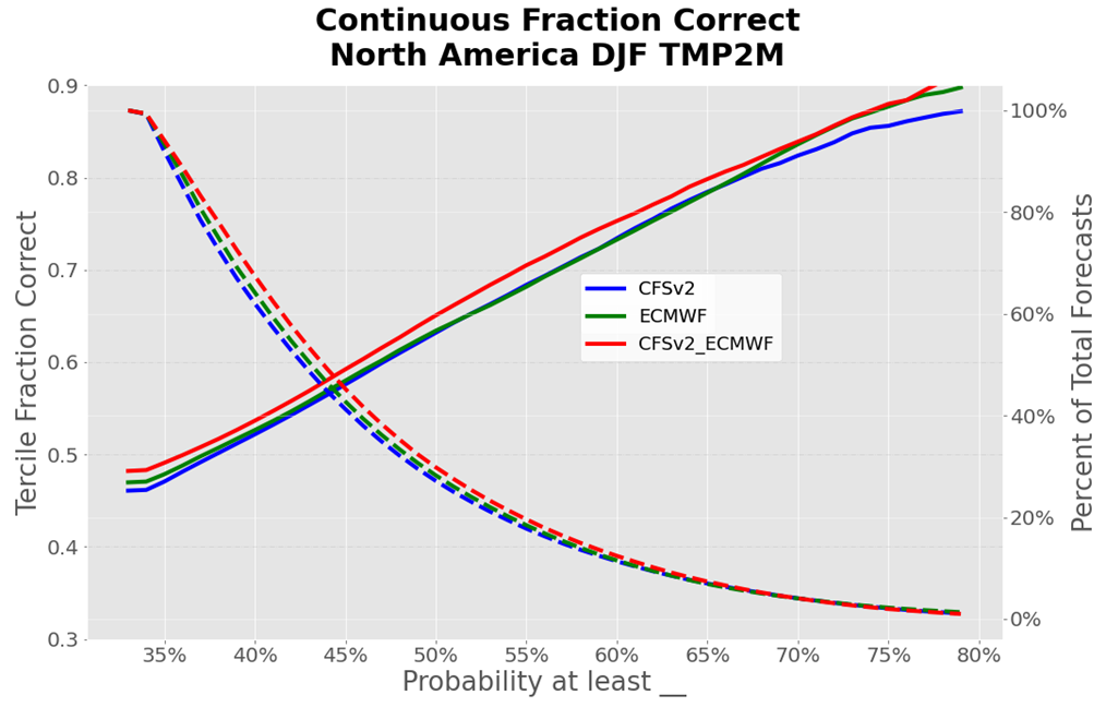
A Multi-Model Ensemble Is comprised of a set of independent dynamical model forecasts. Experimentation has found that when the forecasts of two or more numerical weather prediction models are combined, then the resulting ensemble forecast is usually more skilful than any one individual model Figure 4).
Combining the output from several models is no easy task. Different dynamical models typically employ different modelling parameterization such as grid resolution, and represent physical processes in different ways.
Scientists at the World Climate Service are uniquely experienced in combining dynamical model output whilst ensuring data integrity is maintained. The WCS Multi-Model Ensemble (MME) currently combines the ECMWF and CFSv2 models to produce a more skilful forecast. The WCS will soon upgrade the MME to additionally include the GEFS model.
Ensemble Forecast: WCS Probability Maps
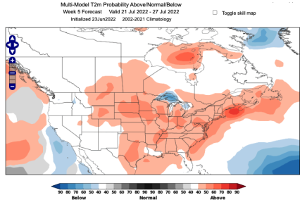
Figure 5 shows an example of a World Climate Service ensemble probability forecast map. Each ensemble member falls into one of the three terciles. The map shows the most likely of the three terciles occurring in a given location. At long lead times, the most probable tercile often has a value below the stringent 40 percent threshold – in which case the map appears blank.
If the most likely forecast tercile probability is 40 percent or greater, the map shade highlights the regions of specific forecast probabilities. In this way, areas with increased probability of specific forecast events are depicted. The example below shows a relatively strong 40-60 percent probability of the Northern US experiencing above normal temperatures five weeks in advance. Conversely, part of Texas is 40-50 percent likely to fall into the below normal category.
Ensemble Forecast: Conclusion
The ensemble forecast consists of many forecasts or members, predicting a range of possible future outcomes. This makes an ensemble forecast more complicated to interpret than a single forecast. However, because the ensemble forecast reflects the initial uncertainty, the range of forecasts produces more skill at longer lead times than a single deterministic forecast.
The range of forecasts produced by the ensemble allows uncertainty to be quantified through a process called calibration. Calibrating the ensemble forecast output creates reliable probabilistic forecasts. The World Climate Service uses calibrated ensemble forecasts to produce subseasonal and subseasonal forecast skill as far as three weeks to six months into the future.