There are two options when delivering a forecast: The forecaster can choose a single value that represents their best estimate of the most likely outcome. This is known as a deterministic forecast. The forecast is unlikely to be perfectly correct, but the forecaster’s objective is to select the most accurate choice among many forecasts.
The second option breaks down the possible outcomes into ranges or bins. A probability of occurrence is assigned to each bin. This is a probability forecast. In this type of forecast, we do not seek to forecast future weather conditions using a specific number. Instead, the probabilistic forecaster seeks to correctly describe the probabilities of the outcome falling in each bin.
It is impossible to say whether a single calibrated probability forecast was correct – it is never right or wrong. Forecasters can, however, gauge how correct (or reliable) probability forecasts are once we have a long enough history of similar forecasts. A reliable probability forecast predicts the probability of specific conditions occurring with the same frequency that they happen in the real world. In other words, a forecast of above-normal temperature with a 60 percent probability is reliable if the temperature is above normal at least 60 percent of the times a forecast with that probability is issued.
What is a Probability Forecast? Probability Forecast Bins
When using probability forecasts, we can choose the size of each bin. For example, if a wind turbine requires a minimum wind speed of 5 ms-1 to start generation, we could create two bins of 0 to 4.99 ms-1 and five ms-1 and above. We could then assign a forecast probability to each of the two bins. The wind speeds can be above or below 5 ms-1, so the predicted two probabilities must add up to 100 percent.
For a given weather variable, we know the full range of possible future outcomes is highly likely to be described by that variable’s long-term history, known as climatology. As signals in long-range weather forecasting are relatively weak, the World Climate Service splits the climatology into three equally likely categories or terciles: above normal, near normal, and below normal. Figure 1 shows an example of creating terciles in an observed temperature distribution.
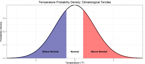
A random number would have a 33.33 percent chance of falling into these three categories. The forecast contains valuable information when the predicted probabilities are not evenly distributed amongst the terciles.
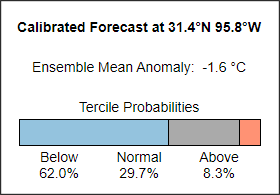
The World Climate Service shows data enabling the user to see the predicted distribution for every point on Earth. An example of the product is shown in Figure 2. Notice how the below-normal, normal, and above-normal categories are not 33 percent but sum to 100 percent.
A forecast framed in terms of probabilities may be difficult for people to interpret as the forecast information includes many possible outcomes. However, the various probabilities provide a convenient input into a numerical contingency model. In other words, a probability forecast allows a user to estimate the risk of different outcomes.
What is a Probability Forecast: World Climate Service Probability Maps
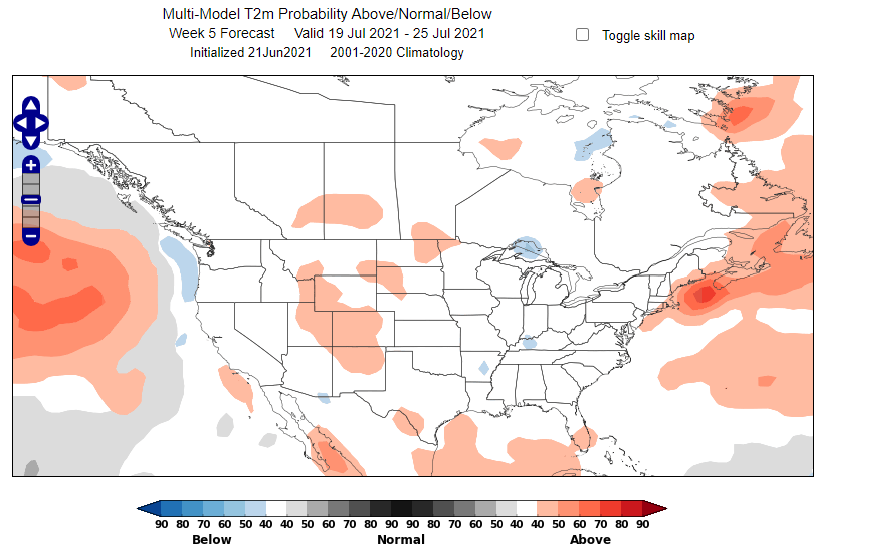
Figure 3 shows a WCS surface temperature probability map with a week two lead time. The map displays only the highest probability for each location when that probability is greater than 40 percent. This threshold is significantly above 33.33 percent, representing a substantially strong signal. This example shows a significant red indication of an 80-90 percent probability of being above normal over the Northwestern US.
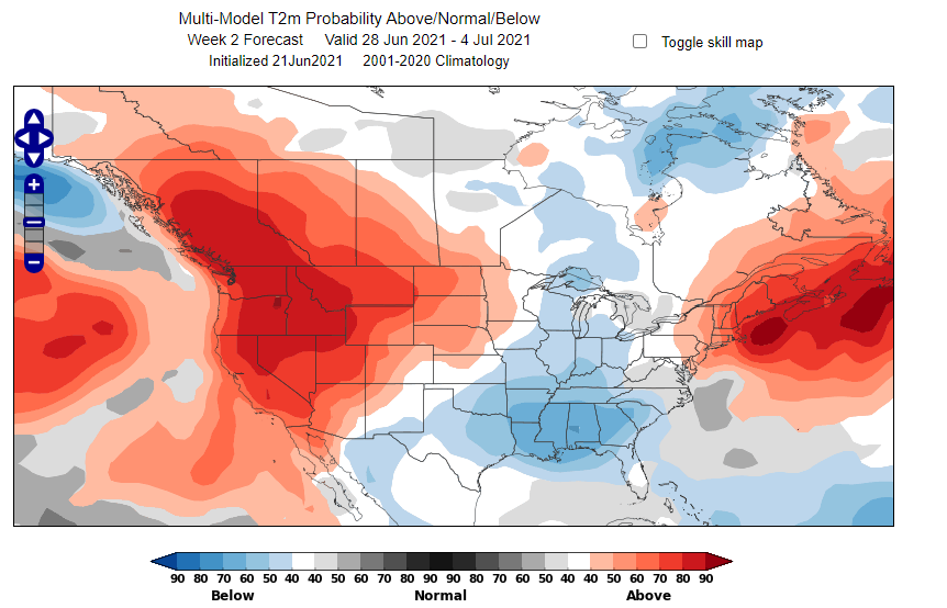
It is important to remember that, despite appearances, this does not tell us precisely how warm it will be, but simply that temperature is highly likely to fall into the above normal tercile.
The map is shaded blue over locations where below-normal temperatures are most likely tercile. The gray shades represent areas where the near-normal tercile is most likely. For statistical reasons, gray shades are less likely to appear than the other colors.
As we move to long forecast lead times, the signals in long-range dynamical forecast models become weaker. As a result, there tends to be less shading on the map. Blank maps can be expected at longer lead times, but they focus the mind on spots where we see a signal in the model.
What is a Probability Forecast: Ensembles
Ensemble forecasting generates many forecasts simultaneously. Each forecast is an equally likely possible future outcome. The output lends itself perfectly to probabilistic forecasting, but the forecasts must be calibrated, and corrections must be applied based on historical forecast performance.
The World Climate Service displays subseasonal ensemble forecasts from ECMWF, GEFS, CFSv2, and the JMA as probability maps. In addition, the WCS combines the output from ECMWF and the CFSv2 to create a “super-ensemble,” or multi-model ensemble (MME).
The World Climate Service displays calibrated long-range forecasts from the CFSv2, ECWMF, UKMO, ECCC, CMCC, DWD, JMA, and Météo-France in the seasonal time frame.
The various models possess different skill levels, and it is observed that the combination of forecasts from different models produces a higher skill than any individual model.
What is a Probability Forecast? Long-Range Forecasting
Long-range forecasts may be highly variable because the uncertainty of the forecast increases with lead time. It is impossible to precisely predict weather variables for a given time and place with lead times greater than around 14 days. However, predicting the likelihood of various outcomes over extended periods is possible. Averaging forecasts over a week in the future reduces the noise that causes forecast uncertainty while extracting the signal that provides predictability. This is why subseasonal forecasts for weeks three to six in the future can be skillful.
As a result, long-range forecasts are framed in terms of the probabilities of specific outcomes, such as below-normal temperatures averaged over a week. WCS probability forecasts have been shown to be skillful surprisingly far into the future.
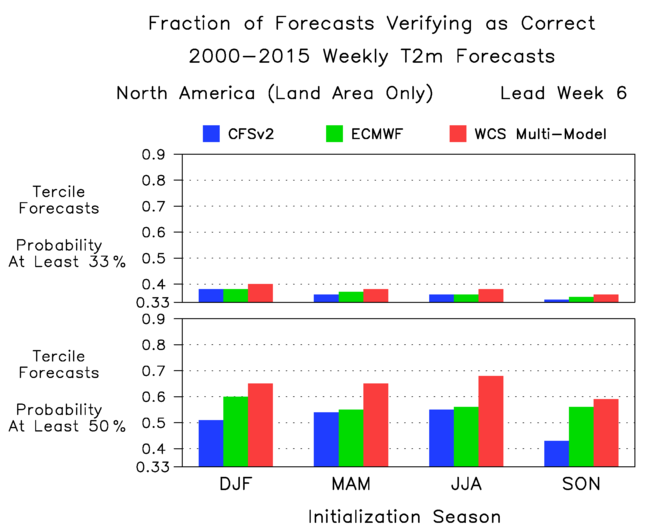
The graphs in Figure 6 show that in lead week six (i.e., a forecast six weeks into the future), when a surface temperature tercile is predicted with a greater than 33.3 percent chance, then that outcome occurs as often as 40 percent of the time (winter, WCS multi-model forecast).
Similarly, in lead week six, when a tercile is predicted with a greater than 50 percent chance, it occurs as often as 68 percent of the time (for summertime forecasts from the WCS multi-model [MME] forecast).
What is a Probability Forecast: Conclusion
Probability forecasts do not seek to predict an atmospheric variable precisely for a given time. Instead, they describe the likelihood of a variable falling into a defined range over a given period of time. This means that probability forecasts are ideally suited to long-range forecasting, where useful signals only appear in ranges over periods of time.
Probability forecasts are also ideally suited to conveying the output of an ensemble forecast comprising a group of similar forecasts.
The skill of a probability forecast cannot be gauged in isolation; it is only when we have a significant number of similar forecasts that we can define their success or reliability.